Write SQL to query MongoDB? You bet!

Are you an experienced SQL sailor navigating new MongoDB waters?

Studio 3T’ has this feature ..

Use familiar SQL statements and operators to view results, and even see the equivalent MongoDB query with Query Code (more on that later).

Get started by clicking SQL in the toolbar, or right-click on any collection and choose Open SQL.

Studio 3T – SQL querying MongoDB

 

 

Basics

There are three ways to open SQL Query:

SQL Query has two main areas: the Editor where queries are written, and the Result Tab where query results are displayed. The other tabs SQL Query, Query Code and Explain will be covered later in the tutorial.

Execute SQL queries

A SQL statement can be executed in three ways:

View the executed SQL query

The SQL Query tab shows which SQL query was executed at cursor.

This is especially useful to confirm which query was actually run, especially in the case of a SQL batch which can contain multiple queries.

In the screenshot above, only the first query appears underneath the SQL Query tab because it is the SQL statement executed at cursor.

Open and save SQL queries

To save the current SQL query as a .sql file, click on the Save icon. Alternatively, click on the arrow next to it to find the Save As function.

To open existing .sql files, click on the folder icon.

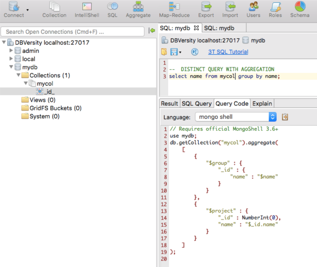
Generate JavaScript, Java, Python and C# code from SQL queries

Query Code is a feature available in Studio 3T that converts SQL queries into JavaScript (Node.js), Java (2.x and 3.x driver API), Python, C#, and the mongo shell language.

To see a SQL query’s equivalent code:

1. Execute the SQL query
2. Click on the Query Code tab
3. Choose the target language

View the equivalent MongoDB query

To view how a SQL query is written in MongoDB query syntax:

1. Click on the Query Code tab
2. Choose mongo shell

Supported SQL expressions

Studio 3T supports many SQL expressions, functions, and ways to express query criteria. This tutorial uses the data set Customers to illustrate examples.

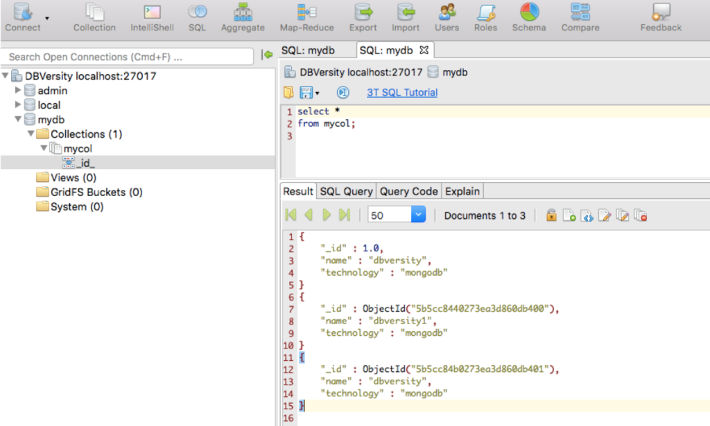
SELECT *

Studio 3T automatically generates a basic SELECT * query by default. This retrieves all of the documents in a collection, similar to selecting all the rows of a table in an SQL database.

The SQL query

select *
from Customers;

shows all documents and fields within the Customers collection.

Access Embedded Fields Using Dotted Names

Some fields may be contained within an embedded document.

In the Customers collection, the field address has four embedded fields: street, city, state, and zip_code.

To find customers living in Berlin, run the following SQL query:

select *
from Customers
where address.city = 'Berlin';

Projection

To see only specific fields (for example, to display only the first name, last name, city, and number of transactions), run the query:

select first, last, address.city, transactions
from Customers;

Comparison Operators

Studio 3T supports the standard SQL comparison operators:  =, <>, <, <=, >=, or >.

To find customers with less than twenty transactions, execute the SQL query:

select *
from Customers
where transactions < 20;

AND or OR

Expressions can be combined using AND or OR:

select *
from Customers
where transactions < 20
and address.city = 'Berlin'
or address.city = 'New York';

ORDER BY

Results can be ordered or sorted by specifying an ORDER BY clause.

By default, ORDER BY sorts results in ascending order, which is the number of transactions in this example:

select *
from Customers
order by transactions;

Add desc to order customers by number of transactions in descending order:

select *
from Customers
order by transactions desc;

Match Boolean Values

Use the Boolean values true and false when querying Boolean fields in a MongoDB document, for example:

select *
from docsWithBoolsCollection
where myBoolField = true;

Some dialects of SQL use the integer values 1 and 0 to represent the Boolean values true and false respectively.

Since MongoDB collections are schema-free, there’s no schema to indicate that a particular field is of Boolean type. Therefore, a value of 1 really means true in that case.

No match will occur when an attempt to match a field with a Boolean value against 0 or 1 is made. With Studio 3T, remember to use true and false when matching Boolean values.

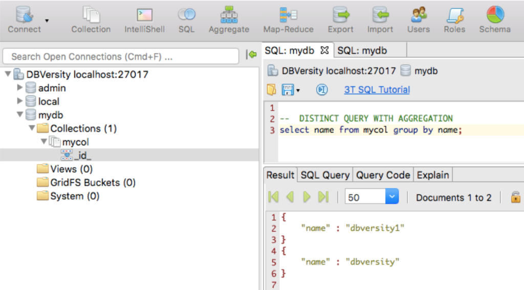
GROUP BY

GROUP BY groups a result set by a particular field, and is often used with other aggregate functions like COUNT, SUM, AVG, MIN and MAX.

For example, to group customers by city, use the following SQL query:

select address.city
from Customers
group by address.city;

The results won’t display the count of customers per city, but the list of unique cities represented in the data.

COUNT

COUNT shows the actual count of documents that match the query criteria.

The following SQL query shows the number of customers per city in ascending order:

select count(*), address.city
from Customers
group by address.city
order by count(*);

SUM

SUM shows the total sum of values of a numeric field.

To see the total number of transactions, execute the query:

select sum(transactions)
from Customers;

AVG

AVG displays the average value of a numeric field across a collection.

The average number of transactions is shown with the query:

select avg(transactions)
from Customers;

MIN

MIN shows the smallest value of a particular field across a collection.

Run the following query to see the lowest number of transactions associated with a single customer:

select min(transactions)
from Customers;

MAX

MAX shows the largest value of a particular field across a collection.

The SQL query

select max(transactions)
from Customers;

shows the highest number of transactions associated with a single customer.

LIMIT

The LIMIT clause limits the number of documents returned in a result set.

Results can be limited to only show 12 customers with the query:

select *
from Customers
limit 12;

OFFSET

The OFFSET clause skips a certain number of documents in the result set.

To skip the first 25 customers while still limiting the results to 12, use the query:

select *
from Customers
limit 12
offset 25;

LIKE

The LIKE operator is stated to find a pattern in the values of a field, often used with wildcards.

Wildcards

Wildcard characters % and _ are used to substitute characters in a string to find matches.

For example:

select *
from Customers
where address.city like '%New%';

will show customers whose cities contain the substring “New”, e.g. Newark, New York, New Orleans.

To show customers whose cities start with the substring “Lon”, the wildcard character % is only placed at the end:

select *
from Customers
where address.city like 'Lon%';

To find customers whose cities start with any letter but ends with “aris”, the wildcard _is used:

select *
from Customers
where address.city like '_aris';

To find customers whose cities that start with any two letters but end with “ris”, simply add an additional _:

select *
from Customers
where address.city like '__ris';

IN

The IN operator can be used to see if a customer is a member of a set.

select *
from Customers
where address.city in ('Berlin', 'New York', 'Wichita');

BETWEEN and NOT BETWEEN

The BETWEEN operator shows if a value lies within a range. The opposite is the operator NOT BETWEEN.

The query to find customers with transactions between 70 to 100 is:

select *
from Customers
where transactions between 70 and 100;

While the query to show customers whose cities start with a letter not in between B and D is:

select *
from Customers
where address.city not between 'B' and 'D';

Special BSON Data Types

MongoDB supports special BSON data types, which in the MongoDB shell are represented by ObjectId, NumberDecimal and BinData, for example.

To query values of these types, write out the values as they would be written in the mongo shell:

select *
from specialBSONDataTypesCollection
where _id = ObjectId('16f319f52bead12669d02abc');

select *
from specialBSONDataTypesCollection
where aNumberDecimal = NumberDecimal('9876543210987654321.0');

select *
from specialBSONDataTypesCollection
where aBinDataField = BinData(0, 'QyHcug==');

ISODate values can also be queried this way, but as described in the section above, it can be more convenient to use the date function provided in the Studio 3T SQL tab to specify date values in various common, concise formats.

Supported SQL joins

Studio 3T built upon MongoDB’s native join functionality and recently introduced support for inner joins and left joins in SQL Query.

Users can write SQL joins, then generate the equivalent Mongoshell code, using the Query Code feature.. They can then use this MongoDB “translation” to query any other appropriate MongoDB database, without additional support or libraries.

However, in doing so, there are one or two considerations to bear in mind, covered below.

Inner joins and left joins

To start, the syntax is simple. To perform an inner join:

select *
from collA
inner join collB on collA.field1 = collB.field2;

And for left joins:

select *
from collA
left join collB on collA.field1 = collB.field2;

Projections

Projections can be performed on the joined collections. These take the following form:

select collA.field1, collA.field3, collB.field2, collB.field4
from collA
inner join collB on collA.field1 = collB.field2;

Note that fields referenced in the projection must be qualified with the collection name, e.g. ‘collA.field1‘ and not just ‘field1‘. While in a relational ‘schemaful’ setting, providing only the column (field) name would be sufficient if it were distinct to one of the tables, in the schemaless MongoDB setting, there’s no schema to indicate to which collection a particular field belongs, so the field name must be qualified explicitly with its collection. By the same token, note that while wildcards such as ‘select * …‘ are permitted, ‘select collA.* …‘ are not.

Multiple joins

Multiple joins are supported, simply write queries such as:

select *
from collA
inner join collB on collA.field1 = collB.field2
left join collC on collB.field3 = collC.field1;

The order in which joins are processed is the same in which they are written, and a join condition must only reference collections to the left of it.

Extended queries

And of course, SQL aggregate functions, group by, having, etc. can all be applied to the joined collections, too:

select collA.field3, collB.field3, count(*)
from collA
inner join collB on collA.field1 = collB.field2
where collA.date > date('2018-01-01')
group by collA.field3, collB.field3
having count(*) > 250
order by collA.field3, collB.field3
limit 1
offset 1;

Joining a collection to itself

A collection can be joined to itself through the use of aliases, for example:

select *
from collA as child
inner join collA as parent on parent._id = child.parentId;

Note that after a collection has been aliased, all references to its fields must use that alias and not the original name.

Cross joins

In case they are needed, cross joins are also supported:

select *
from collA
cross join collB;

or:

select *
from collA, collB;

Take care however, cross join queries can quickly become expensive to run as the number of documents in the collections grow.

Supported date and time formats

Studio 3T allows dates and times to be expressed in a number of different formats.

Although verbose, providing an example of each supported format is the easiest and clearest way of illustrating them.

The supported formats are:

select *
from dates_example
where d > date('2017-03-22T00:00:00.000Z');

select *
from dates_example
where d > date('2017-03-22T00:00:00.000+0000');

select *
from dates_example
where d > date('2017-03-22T00:00:00.000');

select *
from dates_example
where d > date('2017-03-22T00:00:00');

select *
from dates_example
where d > date('2017-03-22T00:00');

select *
from dates_example
where d > date('2017-03-22 00:00:00.000Z');

select *
from dates_example
where d > date('2017-03-22 00:00:00.000+0000');

select *
from dates_example
where d > date('2017-03-22 00:00:00.000');

select *
from dates_example
where d > date('2017-03-22 00:00:00');

select *
from dates_example
where d > date('2017-03-22 00:00');

select *
from dates_example
where d > date('20170322T000000.000Z');

select *
from dates_example
where d > date('20170322T000000.000+0000');

select *
from dates_example
where d > date('20170322T000000.000');

select *
from dates_example
where d > date('20170322T000000');

select *
from dates_example
where d > date('20170322T0000');

select *
from dates_example
where d > date(‘2017-03-22’);

select *
from dates_example
where d > date('20170322');

Ask Question